Water maze strategy analysis with Rtrack

Analysis of spatial search strategies

The Rtrack package is for the analysis of tracking data, as obtained, for example, by the Morris water maze test. The primary motivation was to provide a fast and reproducible way of assigning spatial search strategies to the individual search paths. Based on original ideas from Richard Morris (Morris 1984), automated classification of water maze swim paths was developed by David Wolfer (Wolfer and Lipp 1992) and extended by Graziano et al. (2003) and Garthe et al. (2009) among others since then. This workflow is centred around a new approach using machine learning for swim path classification.

Using ‘Rtrack’ for the Morris water maze

Rtrack aims to provide an easy-to-use interface for the processing of spatial tracking data. This workflow describes analysis of data from the Morris water maze. Assigning a search strategy from a search path is not a straightforward task and a number of approaches have been proposed. Unfortunately, due to the potential complexity of the experiments and the range of computational abilities of the researchers (who are typically experimentalists with little background in programming or data analysis), many existing software solutions have not found their way into laboratory workflows. The Rtrack package is built on the popular and ubiquitous R platform which runs on all commonly-used operating systems, is free and open-source (so that the cost of licencing is not a limitation) and which integrates well into existing analysis environments. The data preparation involves exporting path data from the acquisition software used (outputs from a number of sofware platforms are supported and more are being added), defining the arenas in which the experiment was performed and creating a spreadsheet with information about each track. Once the data and information spreadsheet have been prepared, the actual analysis runs in very little time (processing for 1000 tracks takes under a minute on a typical modern computer) and the data are available in R for further analysis or can be exported for analysis using other software if desired. Publication-quality graphs can be generated and exported directly from the functions in Rtrack. In addition, the raw path data can be saved to a standardised format to allow data sharing and to enhance reproducibility.

About the example experiment

The data provided together with this vignette are from a small pilot study where mice of two strains (‘B6’ and ‘D2’) were trained in a relatively large water maze (190 cm diameter) for 3 days, then tested for a further 2 days after a platform position change (‘goal reversal’). There were 6 trials per animal per day and a total of 5 animals per strain tested. In this particular experiment, the last trial of days 3 and 5 were probe trials—where the goal platform had been removed.

Arena descriptions

An ‘arena’ is a unique combination of a ‘pool’ (or the equivalent for virtual tasks) and the goals—including the goal positions. This means that any change in layout of the arena, or a goal reversal or probe trial, needs to be defined separately in its own arena description file. The description files are simple and consist of only 4–5 lines:

1. The arena type. For a water maze experiment, this will always be mwm
2. The time units. The units in which the timestamps are measured. Each x,y coordinate pair in the path data is associated with a timestamp. The frequency of measurement may be in the range of milliseconds, seconds, hours or even days—depending on the type of experiment. This can either be a text code (‘s’ = seconds, ‘h’ = hours etc.)¹ or a conversion factor to seconds (1 = seconds, 0.0002777778 = hours (a second is 1/3600 of an hour) etc.).
3. The bounds of the arena (i.e. the pool dimensions). This line has four components, each is separated by a space.
   1. The shape. For the Morris water maze, only circle is allowed.
   2. The x coordinate of the arena centre.
   3. The y coordinate of the arena centre.
   4. The radius of the pool.
4. The goal dimensions. Shape, centre x, centre y, radius.
5. The dimensions of the old goal. Shape, centre x, centre y, radius. This is only for reversal trials and does not need to be defined for acquisition trials.

The units for the x and y coordinates do not need to be specified, but these must be the same units used in the raw track files.

For example, the arena description for the example file (‘Arena_SW.txt’) is:

type = mwm
time.units = s
arena.bounds = circle 133.655 103.5381 95
goal = circle 121.8934 154.6834 10

Empty lines are ignored. Any text following the character ‘#’ is also ignored (this allows helpful comments to be embedded into the file).

Assembling the experiment description

The key task before analysing an experiment is to gather together all the information you need for the analysis. This is always necessary for any analysis, and is always a nasty task. Nevertheless, Rtrack uses a straightforward spreadsheet format to make this task less tedious and less confusing.

Several columns are required, these all must begin with an underscore ’_’:

• _TrackID is a unique identifier for each track. The easiest way to do this is just write “Track_1” in the first cell and drag to fill the whole column using Excel’s autofill feature.
• _TargetID is a unique identifier for each subject. Here you should put the animal ID tags, blinded patient IDs or whatever identifies the subjects.
• _Day indicates the day of the experiment. Ideally, use numbers (e.g. 1 for the first experimental day).
• _Trial indicates the trial number. Typically there will be multiple trials per day, but this is not necessary. The field is still required even if a one-trial-per-day paradigm is used.
• _Arena is the name of the arena description file that applies to this track. This is a file path and is relative to the project directory (which is defined by project.dir in the read_experiment function. See the note on relative paths below.
• _TrackFile is the name of the arena description file that applies to this track. This is also a file path and is relative to the data directory (which is defined by data.dir in the read_experiment function. See the note on relative paths below.
• _TrackFileFormat is the format in which the raw track data is stored. See the package documentation (run ?Rtrack::identify_track_format) for a list of the supported file formats.

You can also add any other columns of factors. In the example the mouse strain has been included as well as whether the track was for a probe trial or not. The ‘Probe’ column is a bit special as it can be used to easily filter out probe trials from some plots. If you have probe trials and wish to use this feature, just add the column as shown in the example (‘Probe’ with a capital ‘P’ and values of ‘TRUE’ or ‘FALSE’ only).

Reading in data

Look at one track to get a feel for the workflow. Firstly an arena definition must be read in. This might be different for different acquisition days. The arena is also differently defined for goal reversal trials. This object has the class ‘arena’.

arena = Rtrack::read_arena("MWM_example/Arena_SW.txt")

There are many different raw data formats. The format of the data files depends on the software they were recorded with, the locale and (sometimes) the computer system they were recorded with. Each format supported by Rtrack has a code, which must be given to the read_path function. Run the function identify_track_format with one of the raw track files to help you determine the appropriate format code for your data.

track.format = Rtrack::identify_track_format("MWM_example/Data/Track_1.csv")
#> ✔ This track seems to be in the format 'ethovision.3.csv'.

The tracks for the example are in the format ethovision.3.csv, we need to pass this information on to the reader function. The arena is also required for reading in the path (to provide calibration information).

path = Rtrack::read_path("MWM_example/Data/Track_1.csv", arena, id = "test",
    track.format = "ethovision.3.csv")

Extracting path metrics

The track path/swim path (of class rtrack_path) can now be used to collect a range of metrics. This results in a list of various secondary variables which can be used for plotting and strategy calling.

metrics = Rtrack::calculate_metrics(path, arena)

Plotting the path

The swim path can be plotted. This representation shows the initial path in red, the direct path to the goal as a yellow broken line and the goal corridor in semi-transparent yellow. The concentric zones (wall, outer wall, annulus, centre) are shown in shades of blue.

Rtrack::plot_path(metrics)

The quadrants are defined such that the goal is centred in quadrant North. These may be shown on the plot.

Rtrack::plot_path(metrics, quadrants = TRUE)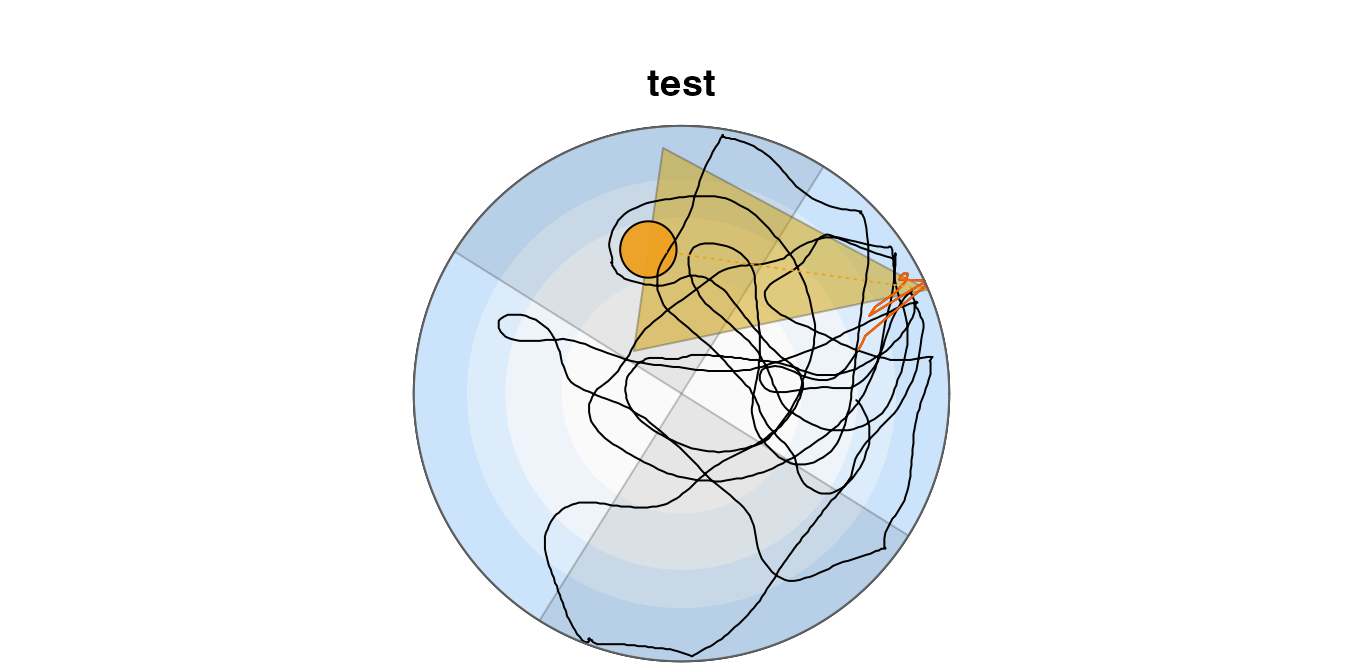

Plotting a density heatmap

Paths can also be plotted as a density heatmap.

Rtrack::plot_density(metrics)

Feel free to play with the colours (just please don’t use a garish ‘rainbow’ scheme). The colour scales are best defined using the ‘colorRampPalette’ function.

Rtrack::plot_density(metrics, col = colorRampPalette(c("yellow", "orange", "red"))(256))

You can use any of the colour definitions provided in R, and reducing the number of colours in the palette gives a contour effect.

Rtrack::plot_density(metrics, col = colorRampPalette(c(rgb(1, 1, 0.2), "orange",
    "#703E3E"))(8))

Calling the strategy

The search strategy can be called using the rtrack_metrics object. For more information on spatial search strategies and the strategies defined in Rtrack, see the associated strategy description page. The default method uses a random forest model trained on several thousands of expert-called search paths.

strategy = Rtrack::call_strategy(metrics)

The resulting rtrack_strategy object contains various information; the actual strategy call can be found in the calls component. A confidence score is an indicator of how well the path fit the model (1 = perfect).

strategy$calls
#>   strategy     name confidence          1          2         3         4
#> 1        4 scanning  0.4415385 0.04769231 0.08461538 0.3169231 0.4415385
#>            5    6 7 8          9
#> 1 0.07846154 0.02 0 0 0.01076923

Reading in experiment data and metadata

The experiment information is read in using metadata in a spreadsheet. See ‘Preparing the input files’ above for details on how to properly construct this file. The raw data are read in, metrics calculated and returned in a list object of class rtrack_experiment. This is the most processor-intensive part of the workflow and an experiment will typically consist of many hundreds of tracks. Depending on the size of the experiment and the speed of your computer, this step may take several minutes (a friendly progress bar will let you know if there is time for a coffee at this step).

experiment = Rtrack::read_experiment("MWM_example/Experiment.xlsx", data.dir = "MWM_example/Data")
#>     Processing tracks.

Parallel processing

It is trivial to parallelise this potentially time-consuming step (if perhaps you have run out of coffee). Now try running the read_experiment code again and see if this makes a difference in processing time.

experiment = Rtrack::read_experiment("MWM_example/Experiment.xlsx", data.dir = "MWM_example/Data",
    threads = 0)

Bulk strategy calling

The strategies can then be called for each track. The strategy-calling methods also take lists of rtrack_metrics objects, or even the whole rtrack_experiment object.. The core strategy-calling method employs vectorised code and is quite fast.

strategies = Rtrack::call_strategy(experiment)

The resulting rtrack_strategy object contains, among other information, all the strategy calls combined in a data.frame.

head(strategies$calls)
#>         strategy            name confidence           1           2           3
#> Track_1        4        scanning  0.4415385 0.047692308 0.084615385 0.316923077
#> Track_2        6 directed search  0.4923077 0.000000000 0.001538462 0.000000000
#> Track_3        4        scanning  0.4661538 0.049230769 0.066153846 0.238461538
#> Track_4        1     thigmotaxis  0.6338462 0.633846154 0.029230769 0.210769231
#> Track_5        6 directed search  0.6830769 0.000000000 0.007692308 0.003076923
#> Track_6        6 directed search  0.7446154 0.001538462 0.018461538 0.000000000
#>                  4           5          6           7           8           9
#> Track_1 0.44153846 0.078461538 0.02000000 0.000000000 0.000000000 0.010769231
#> Track_2 0.01076923 0.006153846 0.49230769 0.418461538 0.067692308 0.003076923
#> Track_3 0.46615385 0.100000000 0.05846154 0.001538462 0.000000000 0.020000000
#> Track_4 0.11538462 0.010769231 0.00000000 0.000000000 0.000000000 0.000000000
#> Track_5 0.07384615 0.033846154 0.68307692 0.195384615 0.003076923 0.000000000
#> Track_6 0.11230769 0.055384615 0.74461538 0.061538462 0.001538462 0.004615385

Analysis of selected metrics

Individual metrics might be of interest for separate analysis; e.g. path length. Here, the path length has been split by mouse strain (a factor in this example experiment).

Rtrack::plot_variable("path.length", experiment = experiment, factor = "Strain",
    factor.colours = c(B6 = "#d40000ff", D2 = "#0169c9ff"), exclude.probe = TRUE,
    lwd = 1.5)

Note that the probe trials have been omitted from this plot.

The ‘summary.variables’ element shows all the metrics available

experiment$summary.variables
#>  [1] "path.length"              "total.time"              
#>  [3] "velocity"                 "distance.from.goal"      
#>  [5] "distance.from.old.goal"   "initial.heading.error"   
#>  [7] "initial.trajectory.error" "initial.reversal.error"  
#>  [9] "efficiency"               "roaming.entropy"         
#> [11] "latency.to.goal"          "latency.to.old.goal"     
#> [13] "time.in.wall.zone"        "time.in.far.wall.zone"   
#> [15] "time.in.annulus.zone"     "time.in.goal.zone"       
#> [17] "time.in.old.goal.zone"    "time.in.n.quadrant"      
#> [19] "time.in.e.quadrant"       "time.in.s.quadrant"      
#> [21] "time.in.w.quadrant"       "goal.crossings"          
#> [23] "old.goal.crossings"

Bulk density maps

It is also possible to create a density heatmap for many tracks together.

Rtrack::plot_density(experiment$metrics)
#> Warning in Rtrack::plot_density(experiment$metrics): Multiple arena definitions
#> have been used. A merged plot may not make sense.

The warning tells us that there are data from tracks using different arenas in our ‘metrics’ list. This almost certainly does not make sense.

However, it might be interesting to look at all the reversal tracks and compare this between the different strains

b6.reversal.metrics = experiment$metrics[experiment$factors$Strain == "B6" &
    (experiment$factors$`_Day` == 4 | experiment$factors$`_Day` == 5)]
d2.reversal.metrics = experiment$metrics[experiment$factors$Strain == "D2" &
    (experiment$factors$`_Day` == 4 | experiment$factors$`_Day` == 5)]
par(mfrow = c(1, 2))
Rtrack::plot_density(b6.reversal.metrics, title = "B6 reversal")
Rtrack::plot_density(d2.reversal.metrics, title = "D2 reversal")

par(mfrow = c(1, 1))

Strategy plots

The strategies can be visualised as contingency plots per trial. Here two plots are made, one for each strain/factor level.

Rtrack::plot_strategies(strategies, experiment = experiment, factor = "Strain",
    exclude.probe = TRUE)

The last function produced two plots. These can be best saved as a multi-page PDF.

pdf(file = "Results/MWM_Strategy plots.pdf", height = 4)
Rtrack::plot_strategies(strategies, experiment = experiment, factor = "Strain",
    exclude.probe = TRUE)
dev.off()
#> agg_png 
#>       2

Plotting all paths

This next block of code produces a large PDF (one page for each track) including each of the paths and titled with the track ID and called strategy. This can be used to check the strategy against your visual interpretation of the path—did our software get it right?

pdf(file = "Results/MWM_Strategy call confirmation.pdf", height = 4)
for (i in 1:length(experiment$metrics)) {
    Rtrack::plot_path(experiment$metrics[[i]], title = paste(experiment$metrics[[i]]$id,
        strategies$calls[i, "name"]))
}
dev.off()
#> agg_png 
#>       2

There are many paths that are very difficult to call (even for a human) and often people will have different interpretations of which strategy is appropriate. The machine-learning method might not always get it ‘right’—but it is consistent. And that can only help reproducibility. We would be interested to hear from you if Rtrack does not perform well with your data. It may be possible to extend the package to cope with a wider range of data sources. See the help page for details on how to contact us.

Thresholding call confidence

The machine-learning algorithm (call_strategy) never outputs a 0 or ‘unknown’ call. It will always assign a call based on the best match to the model. Sometimes these ‘best matches’ are actually rather poor. It may be of interest to use a confidence threshold and discard calls that are below a certain value. We have observed during testing that confidence scores above 0.4 are typically accurate and reproducible, but some paths may not reach this level. It is possible to perform the thresholding easily using the threshold_strategies function.

The thresholded experiment is a new rtrack_experiment object and contains all the same components. The following example uses a confidence threshold of 0.4 and checks the size of the resulting data.frame of strategy calls.

dim(Rtrack::threshold_strategies(strategies, 0.4)$calls)
#> [1] 243  12

It can be seen that only 205 tracks remain at this threshold.

The remaining strategies can be plotted as a strategy plot. The missing values are simply shown as white background.

Rtrack::plot_strategies(Rtrack::threshold_strategies(strategies, 0.4), experiment = experiment,
    factor = "Strain", exclude.probe = TRUE)

As a data.frame

To get a data.frame containing all the experiment metadata, metrics and strategies for each track, it is possible to export the experiment results. The function export_results will, if no filename is given, return the data as a data.frame.

results = Rtrack::export_results(experiment)

Writing to file

The results can also be written to file in any one of several formats. The format will be determined from the filename extension. The default, and most likely to be used in an experimental workflow, is the Excel ‘.xlsx’ format.

Rtrack::export_results(experiment, file = "Results/MWM_Results.xlsx")

Also supported are comma-delimited values (‘.csv’, or ‘.csv2’ where decimal commas are needed) and tab-delimited text (any of ‘.tsv’, ‘txt’, ‘.tab’). You can actually use any file extension, but it will be written in that case as tab-delimited text and you’ll get a warning.

Exporting strategies

The strategy calls can easily be bundled with the other results. Rtrack will make sure that the strategies are in the same order as the results and will pad the strategies with NA where appropriate in case they don’t match the tracks in the results data.frame.

Rtrack::export_results(experiment, strategies, file = "Results/MWM_Results.xlsx")

Exporting a subset of the results

It is also possible to only export some of the results. To do this, just specify the indices or names of the tracks you would like to export.

# Export just the data for strain 'B6'
b6 = experiment$factors$Strain == "B6"
Rtrack::export_results(experiment, tracks = b6, file = "Results/MWM_ResultsB6.xlsx")

Or you may wish to only export tracks with an above-threshold strategy call.

thresholded = Rtrack::threshold_strategies(strategies,
    0.4)
Rtrack::export_results(experiment, strategies, tracks = rownames(thresholded$calls),
    file = "Results/MWM_ResultsThresholded.xlsx")

It is worthwhile noting that the order of the exported results is also determined by the order of the values given to the tracks parameter.

ordered = order(strategies$calls$strategy, decreasing = TRUE)
Rtrack::export_results(experiment, tracks = ordered, file = "Results/MWM_ResultsOrdered.xlsx")

As an RData archive

The entire rtrack_experiment object can easily be saved and reloaded into a later R session. The .RData format is a compressed version of the rtrack_experiment object and requires very little space.

save(experiment, file = "Results/MWM_experiment.RData")

Load the file again (not necessary in this session, but the folowing line demonstates the command needed to read in the .RData file we just created).

load("Results/MWM_experiment.RData")

As a standardised “trackxf” archive

We have also developed a format for saving the raw data in a way that it can be accessed by other software. This allows sharing with other people and archiving in a way that is more likely to be readable in the future. The command below will create a file with the extension .trackxf—you do not need to add the extension though (in fact it is better not to) as Rtrack will take care of naming the file correctly.

Rtrack::export_data(experiment, file = "Results/MWM_example")
#>     Creating trackxf archive.
#>     Compressing trackxf archive.

Data saved in this way can be read back into Rtrack using the read_experiment function (with the format trackxf, although Rtrack will work this out for you). Because only the raw data are saved in trackxf, recreating an experiment in this way will re-calculate all of the Rtrack-specific metrics.

recreated.experiment = Rtrack::read_experiment("Results/MWM_example.trackxf",
    threads = 0)
#>     Restoring archived experiment.
#>     Initialising cluster.
#>     Processing tracks using 8 threads.

This experiment object recreated from the saved trackxf file is (almost) identical to the original object. Only the export information will obviously be different.

# If we set 'export.note' back to empty, then the objects are the same.
recreated.experiment$info$export.note = experiment$info$export.note
all.equal(recreated.experiment, experiment)
#> [1] TRUE